POLYMER SOLUTIONS AND GELS GROUP
Our group uses rheological and vicosimetric techniques to understand the dynamics of polymeric systems, especially polyelectrolytes. Scattering techniques are used to probe the structure of these systems. For this purpose, we use in-house instruments, as those listed in this section and also carry out experiments at synchrotrons and nuetron sources. Here you can find some information about the various instruments available in our labs and the kind of data that these yield. For some of the techniques a brief outline of the principles underlying the measurements is given, this is still work in progress. In addition to the rheology and scattering equipment, we also have have some conductivity and osmometry equipment to study the thermodynamics of polyelectrolyte solutions. Our other equipment include a high precision density meter, a refractometer, a freeze dryer, phase mapping apparatus, a UV-curing source and ultrasonicators.
If you are interested to use any of these instruments, please reach us at: cvg5719@psu.edu
RHEOLOGY
Kinexus Ultra
This is our main rheometer to study polymer solutions. It is a controlled-stress rheometer which combines high sensitivity, with a minimum torque in steady shear of 1 nNm with an efficient solvent trap, which prevents sample evaporation for moderately volatile solvents.
The following geometries and accessories are available:
- Cone-plate geometries: 40 mm and 60 mm, both with a 1° angle. The 40 mm plate requires ≈ 0.3 mL of sample and the 60 mm around 0.7 mL.
- Double gap geometry - especially suited for volatile solvents or low viscosity samples. The sample volume required ≈ 3 mL.
- Plate/plate geometry - 25 mm diameter
- Cone/plate geometry - 25 and 40 mm diameter
- Immersion cell - allows samples to be measured while submerged in a liquid. This is useful prevent evaporation during the measurement of swollen gels.
The maximum shear rate for low viscosity solutions is a few hundred s-1, before Taylor instabilities set in. The specific value depends on the viscosity and elasticity of the sample and the geometry employed. For concentrated polymer solutions, a few thousand s-1 can be reached before viscous heating and/or sample expulsion become significant. Measurements at higher shear rates can be performed with the m-VROCii rheometer.

MCR302e
This is our main rheometer to study poly(ionic liquid) gels, which usually have glass transition temperatures on the range of -80 to -50°C. As the Kinexus ultra, this is a controlled-stress rheometer. The minimum torque is ≈ 1 nNm in steady shear and 0.5 nNm in oscillatory. The normal force can be varied between -50 N to 50 N.
The following geometries and accessories are available:
- Cone/plate geometry - 50 mm diamter and 1° angle.
- Plate/plate geometry - 25 mm diameter
- Glass Plate/plate geometry - for in situ measurements with UV light
As with the Kinexus rheometer, the maximum shear rates that can be applied are limited, and the m-VROCii can be used to extend the measuring range.
A UV lamp can be connected to the rheometer to study light induced polymerisation or cross-linking processes.

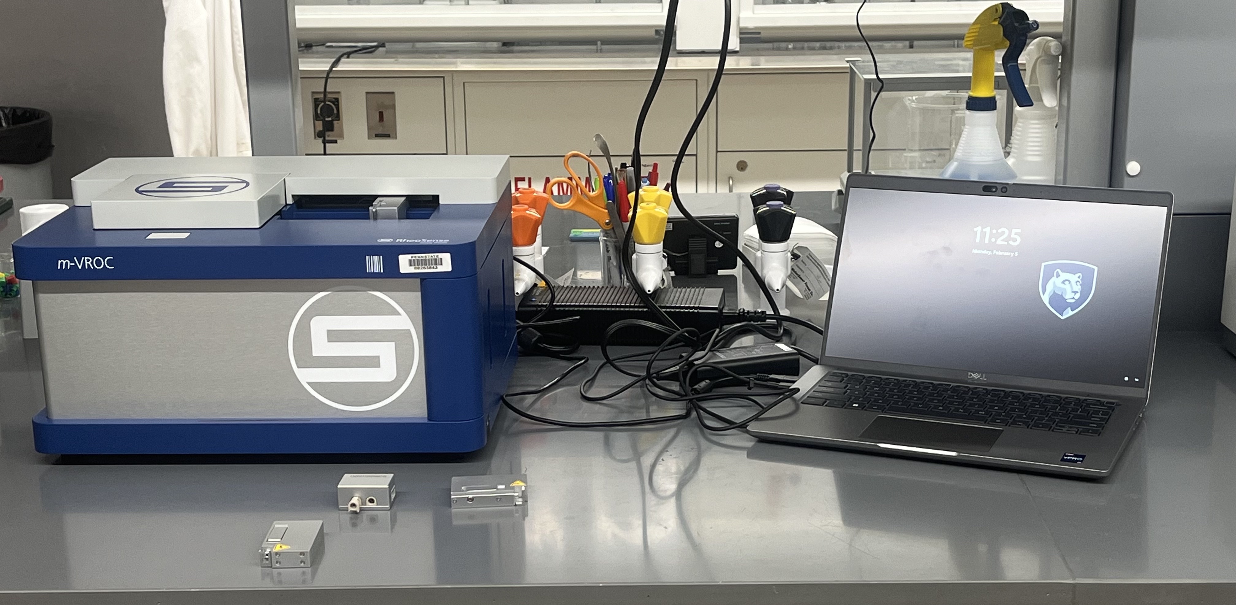
m-VROCii (shear and extensional viscosity)
The m-VROCii is a microfluidic rheometer. TheThe test fluid is flown though a straight channel. The volumetric flow is set by the speed of the pump and the pressure is measured by four pressure sensors at different positions along the channel. The principle of operation is similar to that of capillary viscometers - the main difference being that in the m-VROCii the flow rate is imposed and the pressure measured while in the capillary systems the pressure is imposed (gravimetrically) and the flow rate is measured. Overviews of microfluidic rheometers can be found here and here .
The shear-rate accesible with the mVROCii depends on the chip dimensions and on the viscosity of the samples and can be as high as 2×10⁶ s-1 for low viscosity samples.
Using hyperbolic contraction microfluidic devices, the extensional viscosity of liquids in the range of \(\sim 10^{3}s^{-1}\).
TriPAV- High Frequency Squeeze Flow Rheometer
The TriPAV is a piezo-electric squeeze-flow rheometer. The sample is contained between two metal plates and the lower one is oscillated using a piezo actuator driven by a lock-in amplifier. The accessible frequency range is from 1 to 10,000 Hz. The typical strain amplitude is 0.01-0.2%. A frequency sweep can be carried out over the entire frequency range in under 5 minutes. See this paper for details about the TriPAV performance.
The samples are contained in a hermetically sealed chamber which requires less than 0.1 mL of sample.

Contraves LS-30 (under repair)
The Contraves LS-30 is a cup-and-bob creep rheometer which offers exceptional accuracy for low viscosity samples at low shear rates. This is useful to study non-entangled solutions of high molecular weight polymers, and especially polyelectrolytes in salt-free solvents, where the relaxation time increases upon dilution.

SAMPLE ENVIRONMENTS & ACCESSORIES FOR RHEOLOGY
| Geometry | Instrument |
|---|---|
| Double Gap | Kinexus, DHR30 |
| Cone-Plate | Kinexus (\(\phi = \) 40, 25 mm, 1\(^\circ\)), MCR302e (\(\phi\) = 50 mm, 1\(^\circ\)) |
| Plate-Plate | MCR302e (8-50 mm), DHR30 (25 mm), Kinexus (25 & 40 mm) |
| Couette | Kinexus (double gap), DHR30 (double gap, OSR), Contraves |
| Disposable plates | Kinexus, MCR302e |
| Immersion | Kinexus |
| Equipment | Rheometer |
|---|---|
| Orthogonal Superposition Rheology | DHR30 |
| Rheo-Dielectric Spectroscopy | DHR30 |
| UV-Curing Setup | MCR502/MCR302e |
| Light Scattering | MCR502/MCR302e |
| Environmental Test Chamber | DHR30 |
| DMA: Torsion and Tension | ARES-G2 |
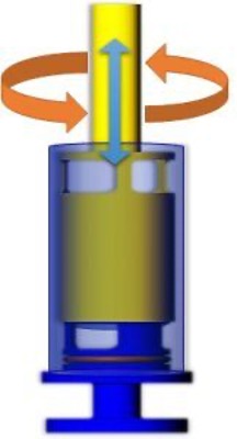
Orthogonal Superposition Rheology
Shear rheology measurements are conventionally carried out either in steady or in oscillatory mode. Steady shear experiments such as creep tests can be used to, for example, evaluate the dependece of the viscosity on shear rate. Oscillatory shear experiments are usually discussed in terms of the loss G\(^{''}\) and storage modulus G\(^{'}\). Orthogonal superposition rheology is a technique which allows for steady and oscillatory shear to be simulataneously applied to a sample. For this, a Couette geometry is used. The bob rotates around its vertical axis (see orange arrows on the figure), imparting steady shear on the sample in the azimuthal direction. Additionally, the bob oscillates in the axial direction (blue arrow), thereby imposing an oscillatory flow in a perpendicular direction to the steady shear.
This setup is available for use with the TA DHR30 rheometer, the temperature is controlled with the Environmental Test Chamber described below. Further details about this technique can be found on the TA website .
Rheo-Dielectric Spectrocopy
A parallel plate geometry, where both plates act as electrodes can be used with the DHR-30 rheometer, combined with the ETC for sample environment control. An oscillating voltage is applied to the plates using the Keysight LCR meter (see below for more details on this instrument). This setup allows us to study the dielectric properties of solutions and gels as a function of applied shear. The Keysight LCR meter has a frequency range of 2Hz-300kHz, which for aqueous polyelectrolyte solutions allows us to measure the conducitivty of solutions but not relaxation processes related to counterion polarisation.
UV-Curing setup
The MCR302 rheometer can be set up with a transparent bottom plate through which UV or visible light of different frequencies can be shone. For details on the Omnicure light source, see below. This setup is particularly useful to monitor cross-linking processes, where the storage modulus and the loss tangent can be related to the degree of cross-linking. For the top geometry, either disposable plates or disposable cones can be used.
Rheo-light scattering
The MCR302e rheometer can be configured in a small angle light scattering (SALS) setup. The light scattered from a sample under flow is measured using a CCD camera.
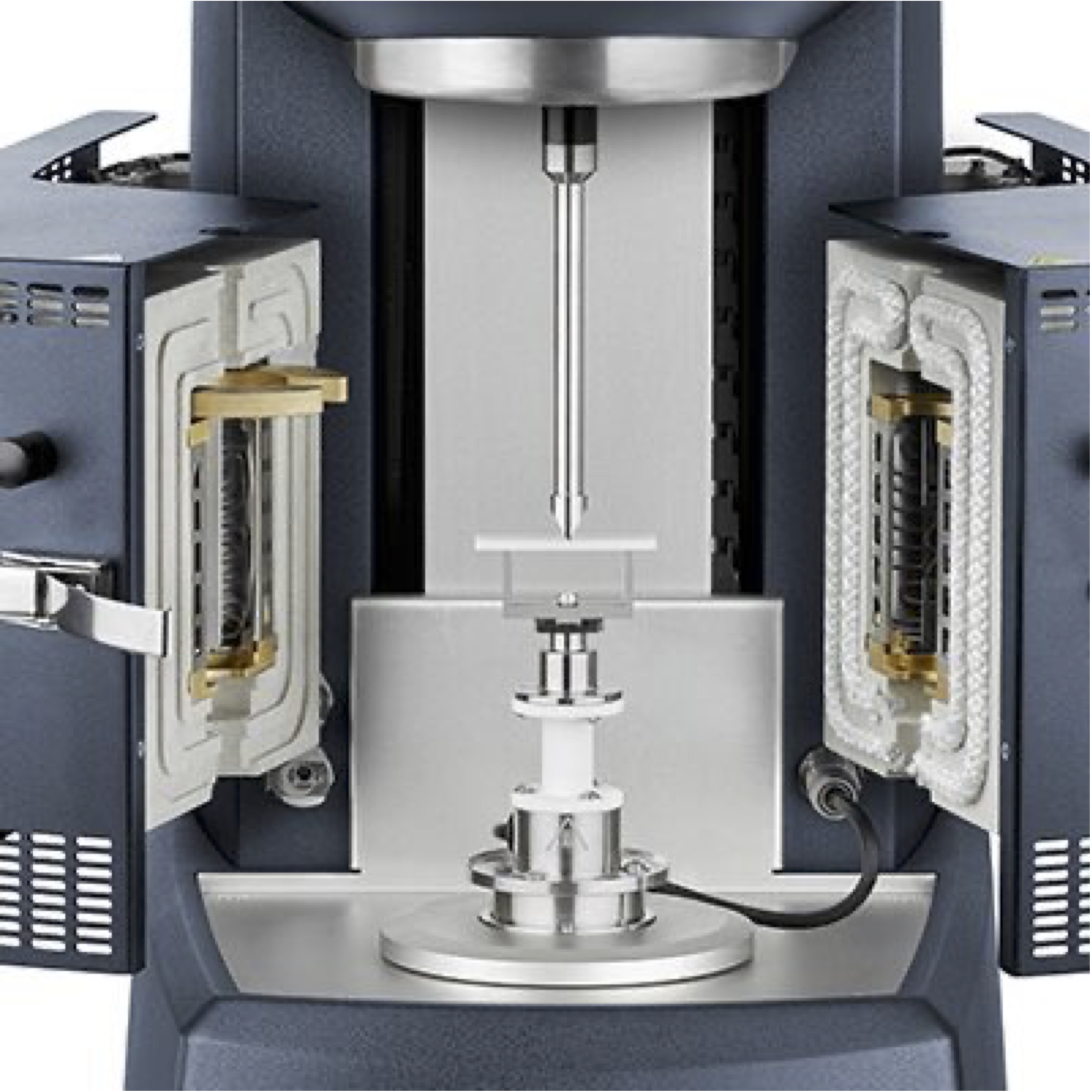
Environmental Test Chamber
The Environmental Test Chamber (ETC), depicted with a DMA accesory on the image to the right, allows the temperature to be changed between -160 °C to 600 using radiant and convective heating. The specific lower temperature ranged is determined by the cooling system employed. Currently, it is set up with the TA Air Chiller System, which can take the ETC down to -80°C without using liquid nitrogen. For lower temperatures, it is necessary to hook up the ETC to a liquid nitrogen dewar. The maximum heating rate of 60 °C/min.
The ETC is used to control the sample enviroment with the orthogonal superposition rheology and dielectric spectroscopy accessories.
Broadly defined, microrheology refers to a series of techniques used to study the mechanical properties of materials at the nanoscale and mesoscale. An overview of the various methods which have been developed over the last two decades can be found here,. A major advantage of microrheological techniques over conventional rotational rheometers is that they can access much higher frequencies. The figure on the right gives a rough estimate of the capabilities of various techniques. Rotational rheometry cannot usually access frequencies larger than ≈100 rad/s. Within that range, it is possible to measure moduly of up to GPa. In DLS-microrheology, samples are loaded with spherical particles with dimaters of a few hundred nanometers. The autocorrelation of the sample is measured and assuming a negligible contribution from the sample, the mean-squared displacement of the particles as a functio of time is calculated. The generalised Stokes-Einstein equation then allows for the storage and loss modulus to be evaluated. Frequencies of up to a few kHz are typically attainable, depending on the sample characteristics. Diffusing wave spectroscopy (DWS) also works by loading the samples with tracer particles, but in this case the concentration is sufficiently high to cause light to be scattered multiple times before it reaches the detector. DWS is usually run in back-scattering geometry. Our lab is equipped with two microheology instruments:
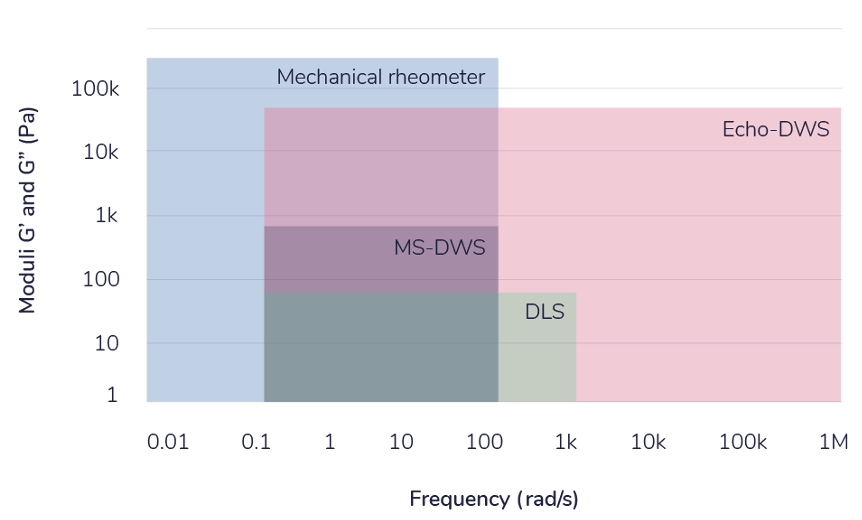
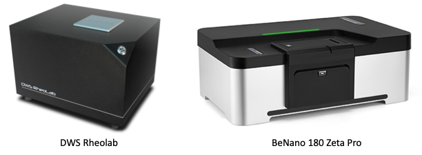
- A DWS rheolab from LS-instruments with the extended frequency option gives access to viscoelastic data for frequencies of up to ≈ 1Mrad/s, depending on sample characteristics. Samples can be measured over a temperature range of 5 to 100 °C and the required volume per sample is between 0.15-1.5 mL, depending on the cell used.
- If samples are loaded with tracer nanoparticles, the BeNanoZeta-pro 180 can be used to run microrheology measurements using DLS. The accessible frequency range depends on the particle size and the sample characteristics. Usually, reliable data can be obtained up to ≈ 10KHz. The sample volume with this instrument can be as low as 50 microliters.
VISCOSIMETRY
EMS-1000S
Samples for the EMS-1000s viscometer contained in a sealed vial, with a metal ball (Aluminium or titanium) is submerged in the liquid. A pair of magnets rotates around the lower part of the vial, causing the ball to rotate. The speed of rotation is recorded and the viscosity of the fluid is calculated. The shear rate range can be varied by changing the speed of rotation of the magnets. The accessible shear rate range depends on the sample's viscosity and the metal ball used. The minimum sample volume required depends on the size of the metal sphere (0.7 mL for \(\phi = 4.7 mm\) and 0.3 mL for \(\phi = 2 mm\)). A low sample volume option is available, which requires only 90 \(\mu L\) of sample. This option works for samples with viscosities in the 0.1-1000mPas range.
A key advantage of this viscometer is that it offers the possibility of measuring samples in a sealed vial. This allows highly volatile solvents to be measured. Samples can also be prepared in a CO\(_2\)-free atmosphere with relative ease.
More information about the instrument can be found on this website.
LOVIS
The LOVIS is rolling ball viscometer where the shear-rate can be controlled by varying the inclination angle. The sample is contained inside a glass capillary and a metal ball, which has a higher density than that of the solution, is allowed to fall down the capillary. The time it takes for the ball to travel through the capillary is measured and used to calculate the kinematic viscosity of the fluid. The inclination can be varied between 15° and 80°, which varies the speed at which the ball travels down the capillary, thereby varying the shear rate. Three capilaries with different internal diameters can be used for measuring samples with different viscosity ranges:
| Capillary ID [mm] | Full angle viscosity range [mPas] | Limited angle viscosity range [mPas] |
| 1.59 | 1-90 | 0.3-20 |
| 2 | 2.5-1700 | 13-300 |
| 2.5 | 70-1700 | 12-10000 |
with the smallest capillary, the shear rate applied can be varied between (200-800/η)s^-1, where η is the viscosity in mPas. Because the speed of the ball travelling down the capillary varies inversely with the solution viscosity, the applied shear rate decreases as the viscosity increases.

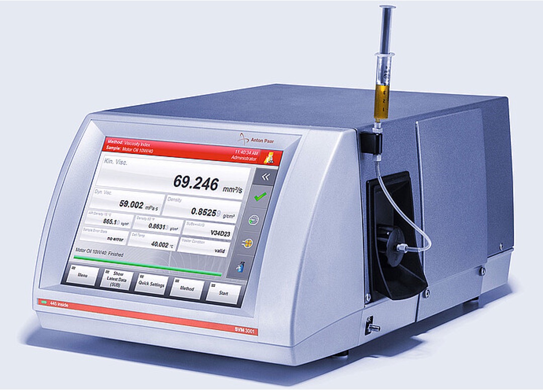
SVM 3001 Cold Properties (Anton Paar)
The SVM3001 instrument is a Stabinger Viscometer. The instrument can measure in the temperatuere range of -60 °C to 100 °C. In addition to the viscosity, the instrument measures the density (reproducibility 0.0001 g/mL), the cloud point (reproducibility ≈ 2.5 °C) and freeze point (reproducibility ≈ 1.3 °C) of fluids. The applied shear rate depends on the viscosity of the sample. As with the LOVIS instrument, the higher the sample viscosity, the lower the shear rate at which the measurement is performed.
This instrument is espcially useful for the determination of the viscosity-temperature curve of oils
Capillary viscometers with automated flow time detection
Measuring principle
For a Newtonian fluid flowing through a capillary, the flow time is given by the Hagen–Poiseuille equation:
\[ Q = \frac{\pi \cdot r^4 \cdot \Delta P}{8 \cdot \eta \cdot L} \]where the symbols have the following meanings:
- Q is the volumetric flow rate
- r is the radius of the capillary
- \(\Delta P\) is the pressure drop across the capillary
- \(\eta\) is the viscosity of the fluid
- L is the length of the capillary
In capillary viscometers, the time taken for a fixed volume of fluid to flow through a capillary of known diameter and length is measured. The flow time (\(t_{flow}\)) can be determined visually or with an automated sensor. The average flow rate is given by the product of the cross-section of the capillary (\(\pi r^2\)) and the average velocity of flow (\(L/t_{flow}\)). The pressure drop across the capillary is a function of the liquid density and viscometer geometry. It is common to express the kinematic viscosity (\(\nu\)) of a fluid as:
\[ \nu = Kt_c \]If end-effects are neglected, \(t_c\) corresponds to the flow time through the capillary, i.e. \(t_c = t_{flow}\). This is a good approximation when flow times are long but becomes increasingly problematic for short flow times, where the 'Hagenbach-Couette' or kinetic energy correction need to be applied, so that \(t_c =t_{flow} - t_{HC} \), where \(t_{HC}\) is a function of \(t_{flow}\). The values of \(t_{HC}\) are provided by the manufacturer for each viscometer type.
The constant K for a given capillary can be determined by measuring a fluid of known viscosity.
For Newtonian liquid (viscosity is independent of the shear rate), the shear rate at the wall of a capillary viscometer can be shown to be:
\[ \dot{\gamma} = \frac{4Q}{\pi r^3} \] where the symbols have the same meaning as above. For typical viscometers, this turns out to be around ~1000 s\(^{-1}\).
Water bath and automatic detection system
A Lauda Brinkmann ECO ER 15 S Waterbath, in combination with an ECO-Gold immersion chiller is used to control the temperature of the bath for the capillary viscometers. Flow times can be recorded manually with the help of a chronometer or using the Lauda automatic iVisc detection system. The iVisc system is controlled with a computer. It can be programmed to draw the solution into the capillary tube, release it, and record the time taken for it to flow down the capillary using an IR sensor. This is typically repated 3-6 times to accurately determine \(t_{flow}\). The iVisc system works with single capillary Ubbelohde viscometers, as shown in the picture above. It cannot be used for other capillary vicometers such as the multiple bulb Ubbelohde or the Cannon-Fieske viscometers. We have a range od different capillary viscometers available in our lab which cover different viscosity ranges and volume requirements. These are listed on the tables below.

Capillary viscometers
Ubbelohde Viscometers
These viscometers require a volume of ≈ 20 mL. They are compatible with the Lauda iVisc automatic detection system.| Type | K [mm²/s²] | viscosity min [mm²/s] | viscosity max [mm²/s] |
|---|---|---|---|
| 0 | 0.001 | 0.3 | 1 |
| 0C | 0.003 | 0.6 | 3 |
| 0B | 0.005 | 1 | 5 |
| 1 | 0.01 | 2 | 10 |
| 1C | 0.03 | 6 | 30 |
Low volume Ubbelohde viscometers
This type of viscometer requires ≈ 1 mL per sample (Cannon viscometers) or ≈ 2 mL per sample (Lauda viscometers). Automatic detection is possible with the Lauda viscometers. We have the following types available in our lab.| Manufacturer | Size | K [mm²/s²] | viscosity min [mm²/s] | viscosity max [mm²/s] | Automatic detection |
|---|---|---|---|---|---|
| Cannon | 25 | 0.002 | 0.4 | 2 | No |
| Cannon | 75 | 0.008 | 1.6 | 8 | No |
| Cannon | 150 | 0.035 | 7 | 35 | No |
| Lauda | I | 0.01 | 0.3 | 6 | Yes |
| Lauda | III | 1 | 30 | 800 | Yes |
Cannon-Manning Semi-Micro Viscometer
This type of viscometer requires only ≈ 0.5 mL per sample. Automatic detection is not possible. We have the following types available in our lab.| Size | K [mm²/s²] | viscosity min [mm²/s] | viscosity max [mm²/s] |
|---|---|---|---|
| 25 | 0.002 | 0.4 | 2.0 |
Shear dilution Ubbelohde viscometers
One of the major drawbacks of capillary viscometers is that they apply relatively high shear rates. For high molecular weight polymers, this means that measurements do not always correspond to the zero-shear rate value. This problem can be partially overcome my using capillary viscometers with varying capillary diameters. For this purpose, we have the following viscometers available, which provide a range of ×10 in shear rate. They can be operated with the same viscometer bath as the other systems. Automatic detection is not possible.
| Catalog no. | Size | K [mm2/s2] | viscosity min [mm²/s] | viscosity max [mm²/s] | shear rate min [s-1] | shear rate max [s-1] |
|---|---|---|---|---|---|---|
| 9723-M50 (x10) | 25 | 0.002 | 0.4 | 2 | 82 | 3300 |
| 9723-M53 (x10) | 50 | 0.004 | 0.8 | 4 | 45 | 1800 |
| 9723-M50 (x5) | 25 | 0.002 | 0.4 | 2 | 82 | 1650 |
| 9723-M53 (x5) | 75 | 0.008 | 1.6 | 8 | 24 | 480 |
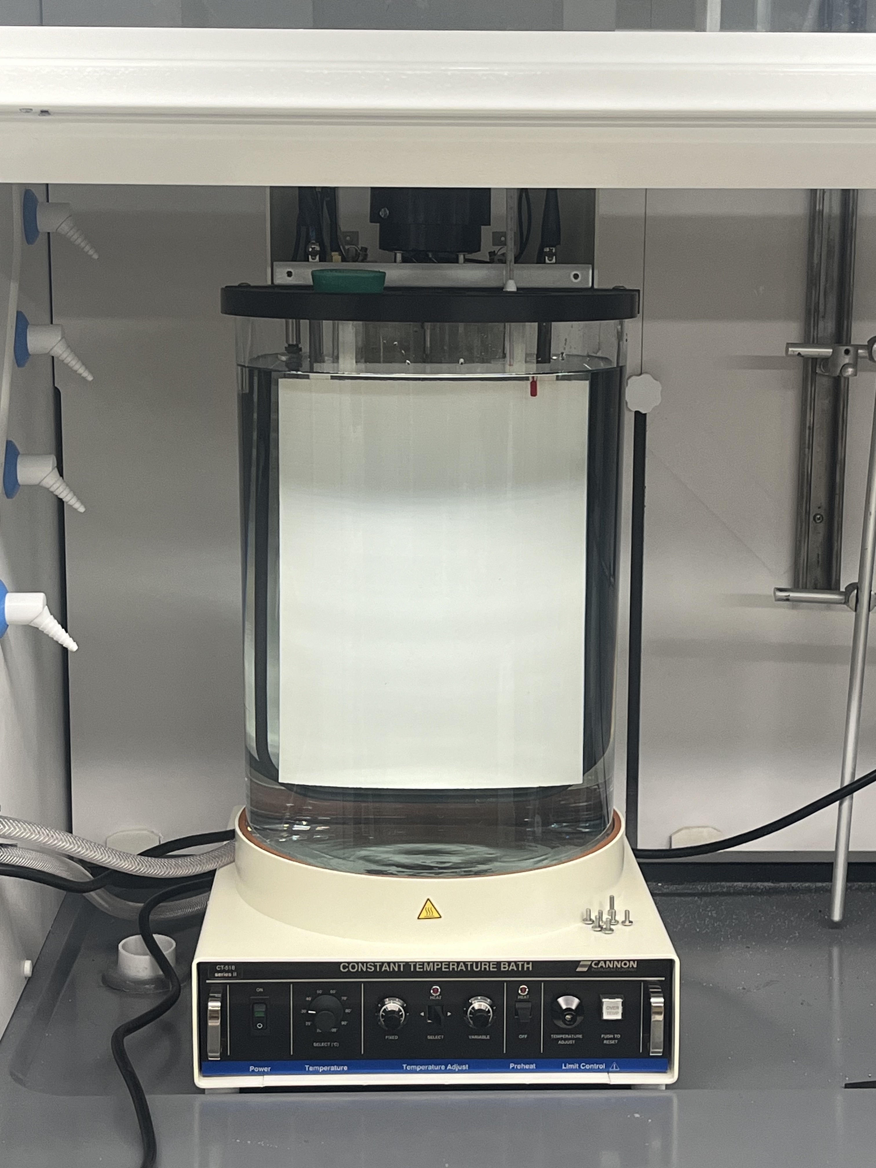
A water bath from Cannon Instrument, model CT-518, in combination with an external water re-circulator allows the temperature of the capillary viscometers to be controlled between 20-100 °C, with a stability of ≈ 0.01 °C. The bath is 46 cm deep, so that long capillary viscometers can be submerged in it. Flow times can be recorded manually with the help of a chronometer.
The table below summarises the various advandtages of the viscometers, considering different performance metrics. Capillary viscometers offer the best accuracy, but this comes at the expense of measuring time and sample volume.
| Instrument | Sample Volume | Viscosity Range | Accuracy | Temperature Range | Measurement Time | Shear Rate Range | Sample Environment |
|---|---|---|---|---|---|---|---|
| EMS-1000S | ≈ 0.3-0.7 mL, (\(90\ \mu L\) with low volume option) | 0.1-100000 mPas | ≈ 3% | 0-200°C, 0-50°C (small sample volume) | < 1 min | Variable | Sealed Environment |
| SVM-3001 Cold properties | ≈ 3 mL | 0.2-30000 mPas | ≈ 1% | 0-100°C (lower T can be extended to -60°C with external chiller) | ≈ 1 min | 1-1000s\(^{-1}\), depends on sample viscosity | Capillary tube |
| LOVIS | ≈ 2 mL | 0.5-90 mPas (upper range can be extended with wider capillaries) | ≈ 1% | ≈ 5-90\(^{\circ}\)C | ≈ 5-30 min, depending on solvent viscosity | 200-800\(^{-1}/\eta\), with \(\eta\) in mPas | Capillary tube |
| Capillary viscometer with automated detection | ≈ 2-20 mL, depending on viscometer | ≲ 10 mPas | ≈ 0.35% | ≈ 20-60\(^{\circ}\)C | ≈ 10-30 min | ≈ 90-2000s\(^{-1}\), depending on viscosity | Open capillary |
| Shear dilution Ubbelohde | ≈ 20 mL | ≲ 10 mPas | ≈ 0.35% | ≈ 20-60\(^{\circ}\)C | ≈ 5-20 min | ≈ 800s\(^{-1}\) | Open capillary |
OSMOMETRY
MEMBRANE OSMOMETERS
Donnan equlibrium of polyelectrolytes

BMT 923
The BMT 923 'onkometer' is a membrane osmometer designed to measure the properties of physiological fluids. The maximum measurable osmotic pressure is 99.9 mmHg or around 13 kPa. For higher osmotic pressures, the osmomanometer can be used. More information about this instrument can be found here.
Wescor 4420 (under repair)
The Wescor 4420 Colloid Osmometer is a membrane osmometer. The maximum measurable osmotic pressure is ≈ 150 mmHg or around 20 kPa. For higher osmotic pressures, the osmomanometer can be used. More information about this instrument can be found on the manual here.
Osmomanometer (under construction)
Membrane osmometers are extremely useful to study the thermodynamic properties of polyelectrolyte solutions. Dialysis membranes are typically permeable to solvent and salt molecules but not to polyelectrolytes. If a polyelectrolyte solution is dialyzed against a salt solution and the osmotic pressure is measured, the polymer contribution to the osmotic pressure can be calculated. This differs from vapor pressure and freeze point depression osmometers, where the oncotic osmotic pressure, which contains contribution from both the polyelectrolyte and salt molecules is measured. Although membrane osmometry was standard characterisation technique in polymer science for several decades, its use has declined. Today, membrane osmometers are not commercially available. Raspaud suggested the construction of a simple osmometer, named the osmomanometer, see this article for details. We are in the process of setting up this instrument.
VAPOUR PRESSURE OSMOMETERS
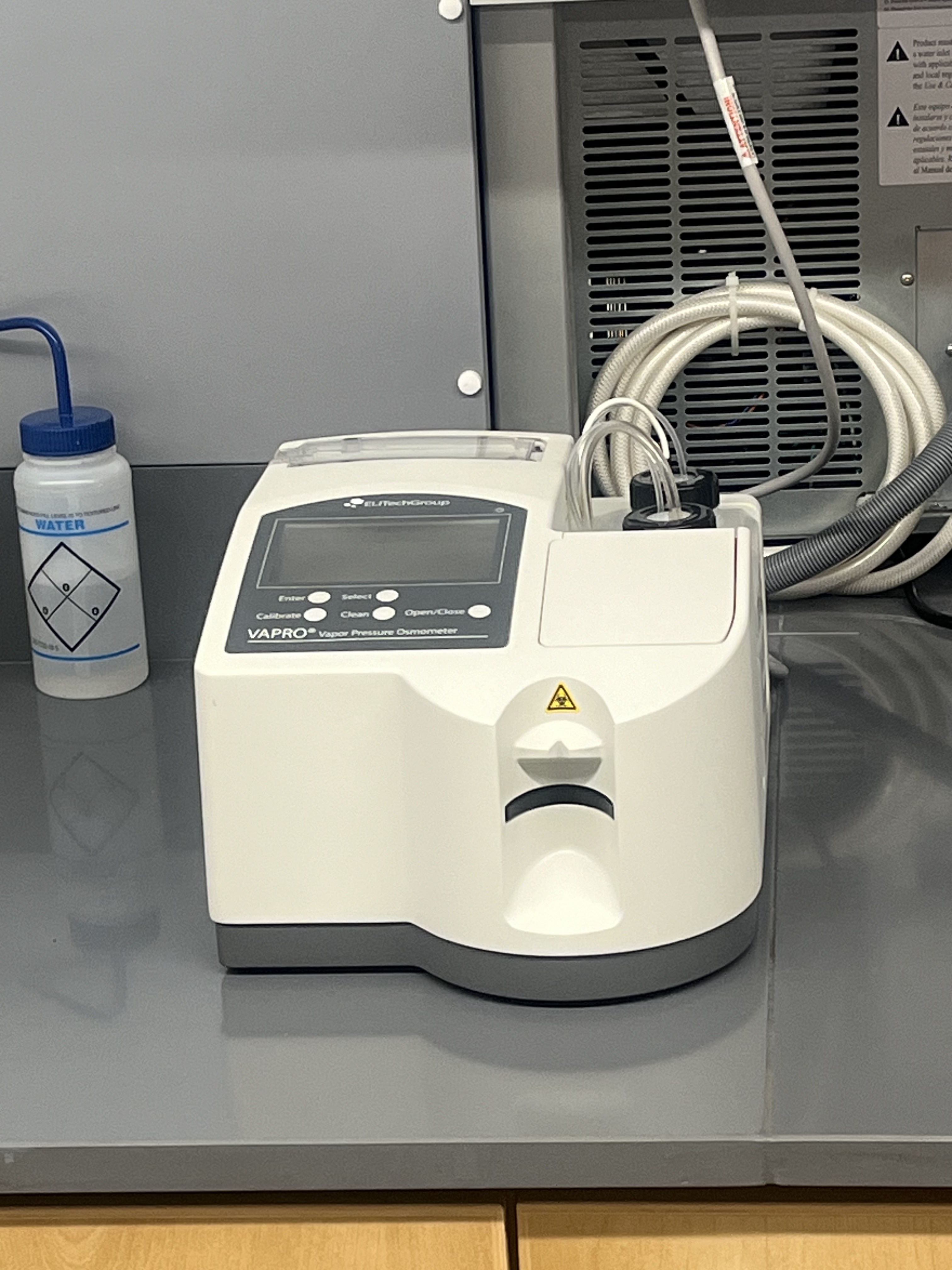
Vapro 5600 osmometer
Our lab is equiped with the Elitech VAPRO 5600 and Wescor 5500 osmometers. Some of the main characteristics are listed on the table below. Literature studies on the osmotic coefficient of polyelectrolytes in salt-free solution using vapour osmometry can be found here , here and here .
| Sample Volume | <0.1 mL. |
|---|---|
| Osmolality range | 0 - 3200 mmol/kg |
| Measurement Time | 90 seconds. |
| Resolution | 1 mmol/kg. |
| Repeatability | 2 mmol/kg Standard Deviation. |
| Linearity | ± 1% of reading over calibrated range (100 mmol/kg - 1000 mmol/kg) ± 5% < 100 mmol/kg and > 1000 mmol/kg up to 3200 mmol/kg ± 10% > 3200 mmol/kg. |
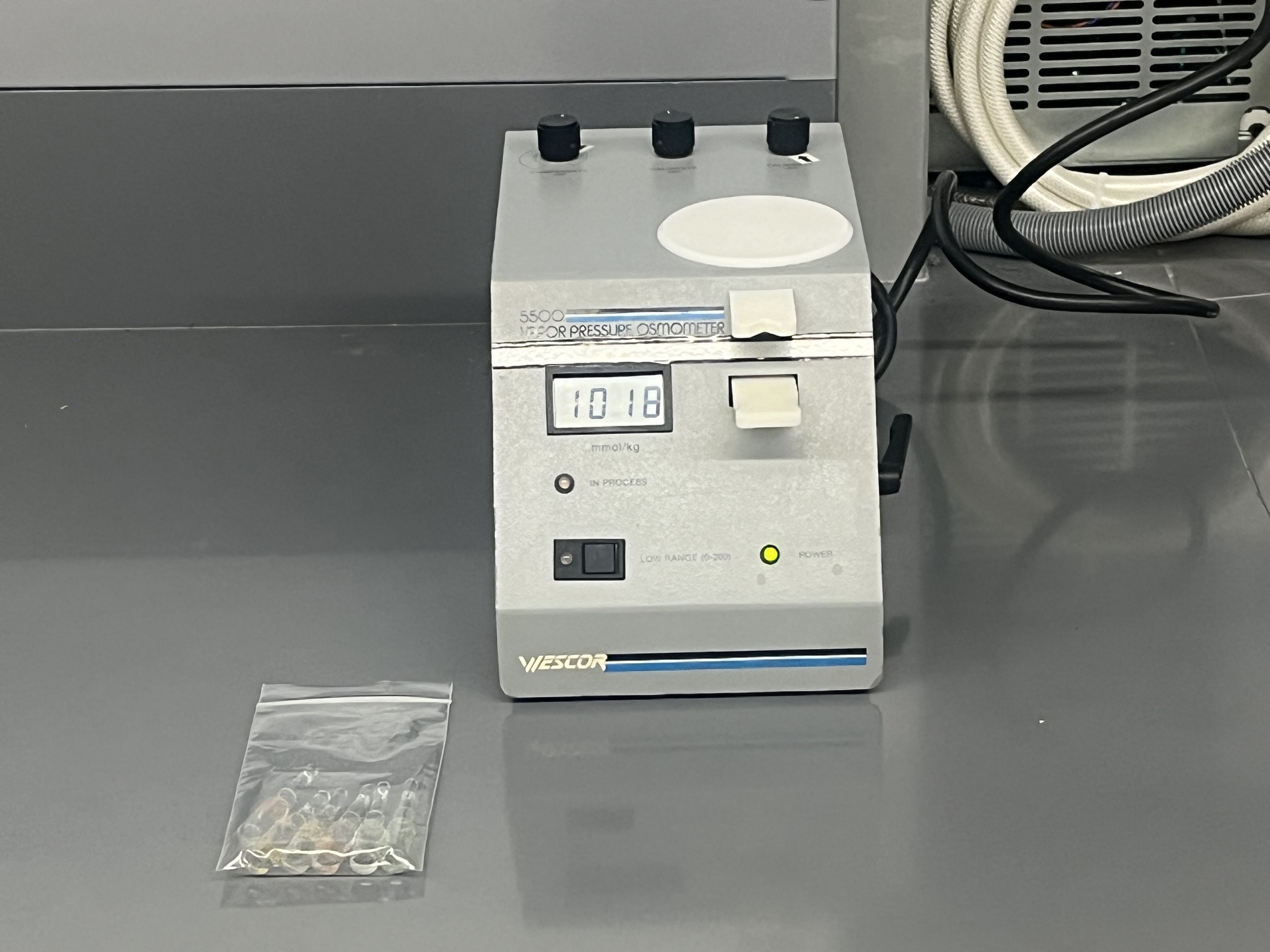
Wescor 5500
This instrument was designed to analyse biological samples. It operates at 37C and works best for high osmolarities (\(\gtrsim 100\) Osm).| Temperature | 37 °C |
|---|---|
| Sample Volume | 10 μL. |
| Osmolality range | 0 - 2000 mmol/kg |
| Measurement Time | 60-90 seconds. |
| Resolution | 1 mmol/kg. |
| Repeatability | 2 mmol/kg Standard Deviation. |
| Linearity | ± 1% of reading over calibrated range (100 mmol/kg - 1000 mmol/kg) ± 5% < 100 mmol/kg |
Knauer K7000 (under repair)
The K-7000 instrument can be used for osmometry of solutions organic solvents. A manual of the instrument can be found here. .| Concentration range | 1 x 10⁻³–15 molal |
|---|---|
| Sensitivity | 3.3 x 10⁻⁵ mol/kg in toluene and 1.7 x 10⁻⁴ mol/kg in H2O |
| Sample volume | approx. 10 µl (one drop) |
| Number of samples | up to 4 samples |
| Test time | 1.5–5 Minutes per measurement |
| Working temperature | 20–130 °C |
| ΔT head thermostat | 0–6 °C |

FREEZE POINT DEPRESSION OSMOMETERS
Freeze point osmometers work by super-cooling a solution several degrees below the freezing point. A mechanical disturbance is then applied to induce ice formation, which is accompanied by the release of heat of fusion. This increases the temperature of the solution until its freezing point. The decrease in freezing/melting point of water (\(\Delta T\)) can be related to the osmotic coefficient of the solution. Specifically, using the crysocopic constant of water of K = 1.858 mK/osmomol, the osmotic coefficient of a solution is: \(\phi = \Delta T/(1.858c) \), where c is the concentration in moles per liter. For an overview of the principles and limitations of freeze-point depression osmometer, see this article.OsmoTECH XT
The OsmoTECH XT is a freeze point depresion osmometer. An advandtage of the OsmoTECH XT over conventional freezeing point osmometers is its ability to handle viscous samples. Details of the instrument performance and sample requirements are listed on the table below.
| Parameter | Value |
|---|---|
| Sample Volume | 20 μL |
| Test Time (Low Range) | ≤150 seconds |
| Test Time (High Range) | ≤190 seconds |
| Resolution | 1 mOsm/kg H₂O |
| Osmolality Range | 0 to 4000 mOsm/kg H₂O |
| Accuracy (0-400 mOsm/kg H₂O) | ±2 mOsm/kg H₂O from nominal value |
| Accuracy (400-1500 mOsm/kg H₂O) | ±0.5% from nominal value |
| Accuracy (1500-4000 mOsm/kg H₂O) | ±1% from nominal value |
| Within-Run Repeatability (0-400 mOsm/kg H₂O) | Standard deviation ≤2 mOsm/kg H₂O |
| Within-Run Repeatability (400-1500 mOsm/kg H₂O) | Coefficient of variation ≤0.5% |
| Within-Run Repeatability (1500-4000 mOsm/kg H₂O) | Coefficient of variation ≤1% |

OsmoTECH 3320
The OsmoTECH 3200 is a freeze point depression osmometer. Details of the instrument performance and sample requirements are listed on the table below.
| Parameter | Value |
|---|---|
| Sample Volume | 20 μL |
| Test Time | 60 seconds |
| Resolution | 1 mOsm/kg H₂O |
| Osmolality Range | 0 to 2000 mOsm/kg H₂O |
| Accuracy (0-400 mOsm/kg H₂O) | ±2 mOsm/kg H₂O from nominal value |
| Accuracy (400-1500 mOsm/kg H₂O) | ±0.5% from nominal value |
| Accuracy (1500-4000 mOsm/kg H₂O) | ±1% from nominal value |
| Within-Run Repeatability (0-400 mOsm/kg H₂O) | Standard deviation ≤2 mOsm/kg H₂O |
| Within-Run Repeatability (400-2000 mOsm/kg H₂O) | Coefficient of variation 0.5% |

Hygro-osmometer (under construction)
Zhan et al proposed a simple idea to measure the osmotic pressure of aqueous solutions using a relative humidity sensor.
SCATTERING
Multi-angle SLS/DLS (Brookhaven)
We use a Brookhaven 2000-BI instrument from Prof. Gomez's lab to study the structure and dynamics of polymers in solution. The instrument is equipped with a red laser (\(\lambda = 633 nm\)) and a green laser (\(\lambda = 532 nm\)). Some characteristics of this instrument are listed below.
Multi-angle SLS/DLS (LSi)
The LSII spectrometer peforms simultaneous static and dynamic light scattering. The pseudocross-corr option allows very short correlation times to be measured compared to the other instruments in our lab. The instrument is useful for the chracterisation of polymers, colloids and other macromolecules such as proteins and antibodies. The table below lists some of the instrument's characteristics:| Parameter | Specification |
|---|---|
| Sample Volume | few mL |
| Particle Size Range (Rh) | 0.15 nm to 5 µm |
| Radius of Gyration | ≈ 10 nm to 1 µm |
| Molecular Weight | 0.360 - 4000 kg/mol (for polymers) |
| Scattering angles |
|
| Angular Resolution | Better than \(\pm\) 0.05° |
| Laser properties | Fiber-coupled laser 120 mW, 638 nm |
| Minium correlation time | 12.5 ns |
| Detectors | Avalanche Photodiode |
| Temperature | 5-90 °C |
Click on the subheadings below to see how the static and dynamic light scattering techniques can be applied to study polymers and polyelectrolytes in solution.
Static light scattering
Static structure factor
One of the most useful equations in scattering relates the structure factor in the zero-angle limit to the osmotic compresibility of the system\[ S(0) = k_BT\frac{dC}{d\Pi} \]
The Zimm Equation
The scattering of dilute polymer solutions in the low scattering wave-vector (\(qR_g \lesssim 1\)) can be modelled using the Zimm equation:\[ \frac{KC}{\Delta R(q)} = \frac{1}{M_w}\Big[1 + \frac{q^2R_g^2}{3}+...\Big] + 2A_2C \]
Here \Delta R is the excess Raleigh ratio (excess means the solvent contribution has been subtracted), C the concentration in mass per volume, M_w is the weight averaged molar mass, R_g^ the squared z-averaged radius of gyration, A_2 the second virial coefficient. K is the contrast factor, given by:\[ K = \frac{4\pi^2n_0^2}{N_A\lambda^4}n\Big(\frac{dn}{dC}\Big)^2_\mu \]
where \(\Big(\frac{dn}{dC}\Big)\) is the refractive index increment of the polymer in the solvent and the subscript \(\mu\) indicates that for three component systems, \(\Big(\frac{dn}{dC}\Big)\) must be determined at constant chemical potential for the diffusible components. For polyelectrolyte solutions, this can be done by performing equilibrium dialysis, see this article. Note that the Zimm equation in the zero-angle limit matches the expression for S(0) given above if the virial expansion for the osmotic pressure is used (\(\frac{\Pi}{k_BTC} \simeq \frac{1}{M} + A_2C+...\)).Semidilute solutions
Above the overlap concentration \(C^*\), solutions are in the semidilute regime. Here the Zimm equation does not apply and instead the scattering intensity is given by:\[ \frac{1}{\Delta R(q)} = \frac{1}{\Delta R(0)}\Big[1 + q^2\xi_{OZ}^2 \Big]\]
here \(\Delta R(0)\) can be related to the osmotic pressure of the system, following the general relation between \(S(0)\) and \(\Pi\) discussed above and \(\xi_{OZ}\) is the correlation length of the system, which is the lengthscale over which concentration fluctuations happen. Understanding the variation of the correlation length with concentration is key to many problems in the statics and dynamics of polymers, see for example chapter 5 of Polymer Physics.
Salt-free polyelectrolytesThe scattering of polyelectrolytes in salt-free solution presents a number of unique features which means that SLS cannot be used to determine their molar mass or radius of gyration in a straightforward manner. However, it is possible to use SLS and DLS to extract useful information on these systems. Below, we will see how these techniques can be used to estimate the fraction of dissociated counterions of a polyelectrolyte. Generally, we can write the osmotic pressure of a polyelectrolyte solution as: \[ \Pi = k_BT\phi c \] here \(\phi \) is the osmotic coefficient and \( c\) the concentration in number of moles of monomers per volume. In semidilute salt-free solutions, each dissociated counterion contributes ≈ \(k_BT\) to the osmotic pressure, so that \(\phi \simeq f \), where <\em>f is the fraction of monomers with a dissociated counterion. As the zero-angle scattering intensity is related to the osmotic compressibility of the sytem, static light scattering provides a way of assessing the effective charge of polyelecrtrolytes in salt-free solution. Often this is complicated by the presence of the so-called low q upturn, which is discussed in the DLS section below. |
Polyelectrolytes & counterion condensationPolyelectrolytes are polymers with ionic groups along the backbone. When they dissolve in a given solvent media, some counterions dissociate from the backbone and go into the bulk of the solution. This leads to a large entropic gain. The rest remain in close proximity to the backbone and are called 'bound' or 'condensed' counterions. These are osmotically inactive. Oosawa and Manning famously predicted that the fraction of condensed counterions of a dilute rod-like polyelectrolyte is: \[f = \frac{b}{l_B}\] where b is the distance between ionic groups on the polyelectrolyte backbone and \(l_B\) is the Bjerrum length: \[l_B = \frac{e^2}{4\pi\epsilon k_BT}\] where \(\epsilon\) is the dielectric constant of the solvent. The Bjerrum length is the distance at which electrostatic attraction between a pair of monovalent charges is equal to their thermal energy. It plays an important role in the solution properties of electrolytes and polyelectrolytes. |
Dynamic light scattering
Dynamic light scattering measures the intensity autocorrelation function \(g_2(t,q)\)
\[ g_2(t,q) = \frac{\langle I(q,t)I(q,0) \rangle}{\langle I(q,t) \rangle ^2} \]The field autocorrelation function is calculated with the Siegert relation: \[ g_2(q,t) = B + \beta [g_1(q,t)]^2 \] where \(B\) is the baseline and \(\beta\) is a coherence factor.
The field correaltion function \(g_1(q,t)\) of a solution monodisperse particles can be modelled by a single exponential decay:
\[ g_1(q,t) = e^{-\Gamma t} \]where \( \Gamma \) is the inverse relaxation time, also known as the first cumulant and \(t\) is the correlation time.
The diffusion second virial coefficient (\(k_D\))
Work in progress...
Measurements are carried out at different angles, and \(\Gamma/q^2\) is extrapolated to \(q \rightarrow 0\):
\[ \frac{\Gamma}{q^2} = D_{app}(1+C'R_g^2q^2) \]
where \(D_{app}\) is the apparent diffusion coefficient, \(R_g\) the radius of gyration and \(C'\) is a dimensionless constant which depends on the size, shape and polydispersity of the solute, see this paper and this paper for more information on how to calculate \(C'\).
Measurements as a function of solute concentration in the dilute regime (\( C\lesssim C^* \)) allow the apparent diffusion coefficient to be extrapolated to the \( C \rightarrow 0 \) limit, which yields the translational diffusion coefficient \(D_0\) of the macromolecule: \[ D_0 = D_{app}(1 + k_DC) \] here \(k_D\) is the diffusion second virial coefficient, which for high molecular weight polymers in the good solvent limit is of the order of \(1/C^*\), see text box on the right. For polydisperse systems, the single exponential expression can be replaced by a modified cumulant expansion:\[ g_2(q,t) = e^{-\Gamma q^2 t} \Big(1 + \frac{\mu_2t^2}{2} + \frac{\mu_3t^3}{6} + ...\Big) \]
where \(\mu_2\) and \(\mu_3\) are the second and third cumulant, respectively. These contain information on the molar mass distribution of the samples. For the relationship between the second cumulant and the polydispersity (\(M_w/M_n\)), see this paper by Selzer. The translational diffusion coefficient of a macromolecule is related to the hydrodynamic radius by the Stokes-Einstein equation: \[ R_H = \frac{k_BT}{6\pi\eta_s D_0} \] where \(\eta_s\) is the viscosity of the solvent.The hydrodynamic radius of a macromolecule is defined as the radius of a sphere with the same diffusion coefficient as that of the macromolecule. The ratio \(\rho = R_g/R_H\) is sensitive to particle shape and polydispersisty. For spheres \(\rho = 0.78\) and for polymers \(\rho \simeq 1.3-2\).
Above the overlap concentration, the equations above can be used to obtain apparent diffusion coefficients \(D\), which can be used to calculate the dynamic screening length (\(\xi_H\)) \[ \xi_H = \frac{k_BT}{6\pi\eta_s D} \]Combined Static and Dynamic light scattering
BeNano Zeta-pro 180
The BeNano Zeta-pro 180 performs three light scattering techniques: static light scattering, dynamic light scattering, and electrophoretic light scattering. For samples such as protein solutions, this allows the particle size, zeta potential, and molecular weight to be determined. Additionally, samples are loaded and the DLS measurement can be used to perform microrheology experiments.
The instrument is equipped with a solid-state 50 mW red laser (λ = 671 nm) and avalanche photodiode detectors. SLS and DLS can be performed at angles of 90° and 173° (backscattering). For small particles such as proteins, for which the scattering intensity is q-independent in the light scattering range, the weight average molar mass and second virial coefficient can be obtained from SLS and the hydrodynamic radius and diffusion virial coefficient can be obtained from DLS.* Electrophoretic light scattering is performed at 12°. In the back-scattering mode, the instrument can perform non-invasive back-scattering, which is useful to prevent multiple scattering in concentrated samples.
*Light scattering at single angle
Usually, to obtain the translational diffusion coefficient of a macromolecule, it is necessary to extrapolate to q = 0. The correlation function measured at a fixed angle gives an inverse decay \(\Gamma\), from which the apparent diffusion coefficient can be calculated as:
\[ D_{app} = \Gamma/q^2 = D(1 + k_Dc)(1 + Cq^2R_g^2) \]where D is the translational diffusion coefficient of the solute, \(k_D\) is the diffusion second virial coefficient, c is the concentration and C is a constnat. In general, if experiments are performed at a single angle, the obtained diffusion coefficient does not match that the translational diffusion coefficient of the macromolecule. There are some exceptions such as monodisperse spheres, for which C = 0. More generally, if \(C(qR_g)^2 \ll 1\), the angular dependence of the diffusion coefficient can be neglected.
The scatteing wave-vector q is: \[ q = \frac{4\pi nsin(\theta/2)}{\lambda}\]In aqueous solution (refractive index \(n ≈ 1.33\) and for a scattering angle of 90°, q ≈ 0.018 nm\(^{-1}$\). For polymers in solution C \simeq 0.2. Therefore, for a polymer with \(R_{g,z} = 20\)nm, \(C(qR_g)^2 \simeq 0.02\), meaning that the diffusion coefficient measured at 90°, after extrapolation to zero concentration, matches the translational diffusion coefficient of the polymer to very good accuracy. On the other hand if \(R_{g,z} = 50\)nm, a measurement at 90° will underestimate the diffusion coefficient by ≈ 15%.
The range over which single-angle light scattering yields accurate results for the diffusion coefficient and molar depends on the specific system because n and C depend on the solvent and solute respectively.
Electrophoretic light scattering
Electrophoretic light scattering (ELS) is a technique that allows the electrophoretic mobility of solute particles to be determined. In brief, the solution is placed between two electrodes and a voltage is applied. This causes charged species to move along in the direction of the electric field. A laser is shone trhrough the sample. When light scatters of a moving particle, it's frequency undergoes a change (Doppler shift). For the velocities of typical macromolecules and colloids under electrophoresis, this shift is too small to be measured directly. The solution is to combine the scattered beam with a beam from the same laser which has not gone through the sample. When light of two frequencies is combined, a beating pulse is generated, from which the original doppler shift can be calculated.
Constant Volume dialysis cells
To obtain the molar mass of polyelectrolytes with static light scattering, the refractive increment difference has to be measured at constant chemical potential for the diffusible components (solvent and salt). Fixed volume dialysis cells are available in our labs for this purpose. They can be used to determine \(\Big(\frac{dn}{dc}\Big)_\mu\) or to measure salt-exclusion Donnan coefficients.Xenocs 2.0 (Materials Characterisation Lab)
We use the Xeuss 2.0 from Xenocs at the Materials Characterisation Lab to study the structure of polyelectrolyte solutions. Additionally, we make a yearly trip to the BL40XU beamline at the Spring-8 synchrotron.CONDUCTIVITY & POTENTIOMETRY
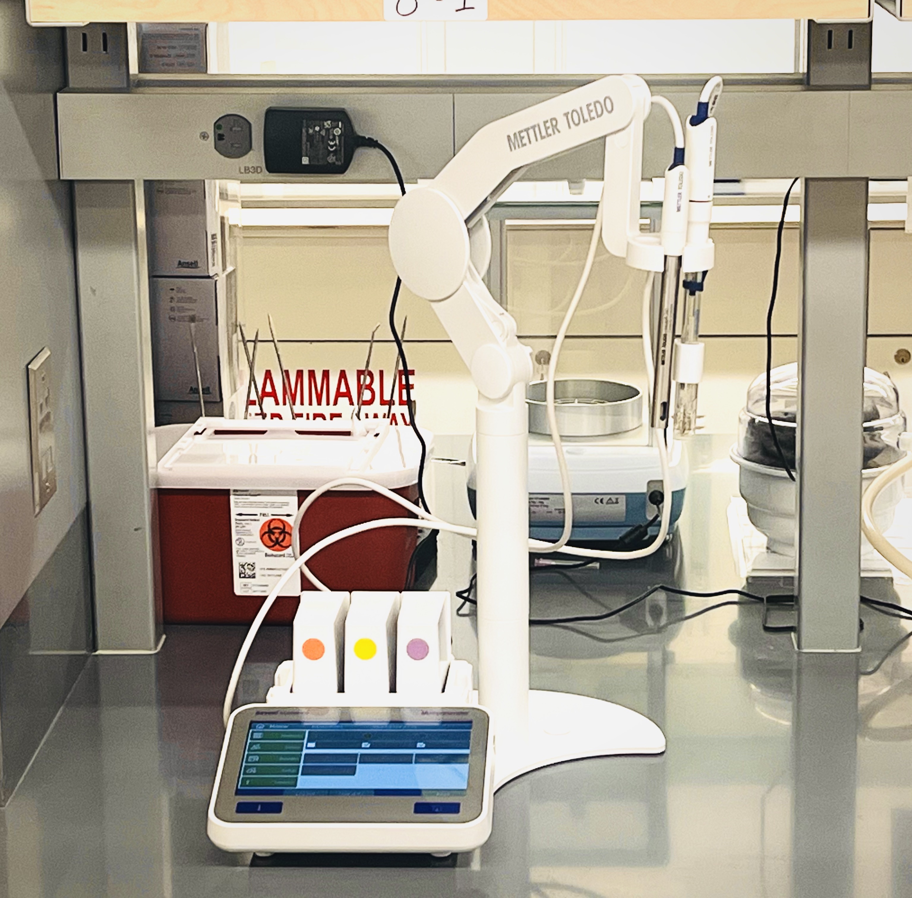
SevenExcellence S475 pH/mV/ION and Conductivity Meter
The SevenExcellence instrument can be used to measure the electrical conductivity and pH of solutions. Additionally, it is possible to use ion-selective electrodes to determine the concentration of different ions. A list of the various probes available can be found in the table below:
| Model number | Type | Notes | Range |
|---|---|---|---|
| INLAB 720 ELECTRODE | Conductivity | 2 platinum poles conductivity cell | 0.1 – 500 µS/cm |
| PROBE CONDUCTIVITY 741 | Conductivity | 2 steel poles | 0.001 – 500 µS/cm |
| INLAB 710 ELECTRODE | Conductivity | 4 platinum poles | 10 – 5×10⁵ µS/cm |
| PROBE CONDUCTIVITY 731 | Conductivity | 4 graphite poles | 10 – 106 µS/cm |
| SODIUM ELECTRODE W/S7 HEAD | Ion Selective electrode | Na+ | 1×10⁻⁷ – 1 mol/L |
| POTASSIUM ELECTRODE WITH BNC | Ion Selective electrode | K+ | 1×10⁻⁶ – 1 mol/L |
| PH ELECTRODE INLAB ROUTINE PRO | pH Electrode | 12 mm shaft | 0-14 |
| INLAB MICRO PRO-ISM ELECTRODE | pH Electrode | 5 mm shaft | 0-14 |
2-electrode cells typically display greater sensitivity and are hence more suited for low conductivity samples, such as solutions in apolar organic solvents. 4-electrode probes are better suited for solutions with higher conductivity and are less affected by electrode polarisation. For salt-containing solutions, the LCR Meter from Keysight should be used to make sure that the conductivity is measured over a frequency range over which electrode polarisation effects are not important.
BeNano Zeta pro 180
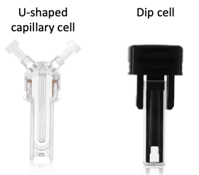
In electrophoretic light scattering mode, the BeNano measures the conductivity of samples by applying an oscillating electric field with a frequency of ≈ 200 Hz. The electrodes are 1 cm apart magnitude of the field can be tuned between 1 and 200 V. Working at low electric fields helps mitigate electrode polarisation. While less precise than the conducitivty meter, conductivity measurements on the BeNano instrument require less sample volume (≈ 1-1.5 mL), and the sample is contained in a sealed environment, thus preventing evaporation. Measurements can be run over a temperature range of 10-70 °C. U-shaped capillary cells are available for aqueous samples and a dip cell is available for organics.
Keysight E4980Al LCR Meter (coming soon)
As mentioned above, electrode polarization can be a problem when studying the conductivity of salt-containing solutions, see this this document, written by Prof. Ralph Colby for a detailed explanation of the phenomenon. The Keysight E4980AL LCR Meter can be used to measure the electrical impedance of solutions to be measured in the range of 20Hz to 300 kHz, which allows the conductivity of solutions to be obtained without electrode polarization effects.
Co-axial liquid cell
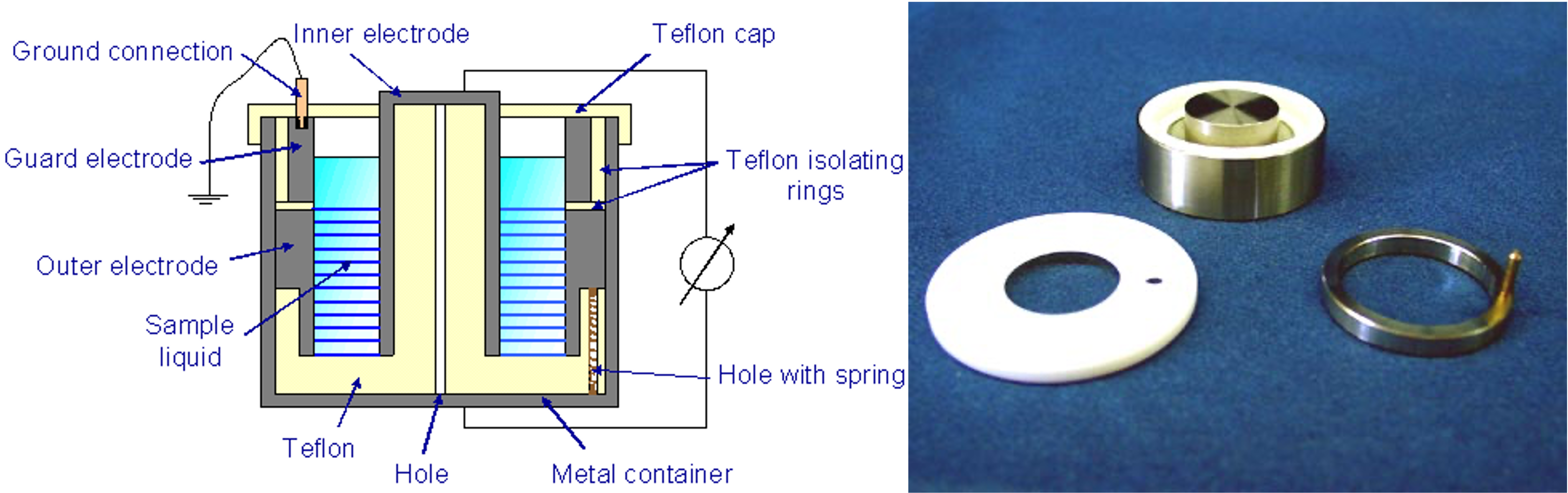
For liquid samples, we have a co-axial cylinder cell from Novocontrol, as shown on the figure to the right. This can be connected to the Keysight LCR meter or the Novocontrol dielectric spectrometer instrument from prof. Colby's lab. The sample volume required using this cell is ≈ 3 mL.
REFRACTOMETERS & DENSITY METERS
Knowing the refractive index increment of polymer solutions is essential for accurate molar mass determination using static light scattering.RA-620 (KEM)
Our Lab is equipped with a RA-620 refractometer by KYOTO ELECTRONICS MANUFACTURING (KEM). Some of the model characteristics are listed below. The instrument also provides the refractive index in terms of the Brix scale, which can be used to estimate the concentration of dissolved sugars in an aqueous solution.| Measuring Method | Detection of Critical Angle of Optical Refraction |
|---|---|
| Light Source | LED Na-D Line (589.3nm) |
| Measuring Range | Refractive Index (n): 1.32000 - 1.58000 |
| Accuracy | Refractive Index (n): ±0.00002 |
| Repeatability & Resolution | Refractive Index (n): ±0.00001 |
| Temperature Range | 5 - 75 °C |
| Temperature Indication Resolution | 0.01°C |
| Minimum Amount of Sample | 0.2 mL |

More information: consult the manufacturer's website.
The refractive index increment varies with laser wavelength according to the Cauchy equation:
\[ \frac{dn}{dc} = A + B \lambda^{-2} \]
where A and B are coefficients which depends on the polymer-solvent pair. The molar mass of the may sometimes have an influence on these coefficients.
BI-DNDC (Brookhaven)
This is a differential refractometer from Brookhaven instruments, operating at a wavelength of 470 nm.| Measuring Method | Detection of Deflection Type refractometer |
|---|---|
| Light Source | 470 nm |
| Measuring Range | Refractive Index (n): 1.00 - 1.75 |
| Accuracy | \(\Delta\)n: ≈ 1.5 \(\times 10^{-3}\) |
| Temperature Range | 25 - 80 °C |
| Temperature Accuracy | 0.1°C |
| Minimum Amount of Sample | ≈ 2 mL |

The same instrument but for \(\lambda = 620\) nm and \(\lambda = 780\) nm are available in the Colby and Gomez labs. Combining the four refractometers, the dn/dc at any range in the visible spectrum can be estimated.
Optilab rEX (Wyatt Technology)
This is a differential refractometer from Wyatt instruments, operating at a wavelength of 690 nm.| Measuring Method | Deflection Type refractometer |
|---|---|
| Light Source | 690 nm |
| Measuring Range | Refractive Index (n): 1.2 - 1.8 |
| Temperature Range | 4 - 50 °C |
| Temperature Accuracy | 0.005°C |
| Minimum Amount of Sample | ≈ 0.1 mL |

2WAJ Abbe Refractometer
| Measuring Method | Detection of Critical Angle of Optical Refraction |
|---|---|
| Light Source | LED Na-D Line (589.3nm) |
| Measuring Range (liquid) | Refractive Index (n): 1.3000-1.7000 |
| Measuring Range (solid) | Refractive Index (n): 1.3000-1.63 |
| Accuracy | Refractive Index (n): ±0.0003 |
| Temperature Range | 0 - 70 °C |
| Temperature Indication Resolution | 0.1°C |

| Instrument | Measuring Method | Light Source | Measuring Range | Accuracy / Resolution | Temperature | Min. Sample |
|---|---|---|---|---|---|---|
| BI-DNDC (Brookhaven) | Detection of Deflection Type refractometer | 470 nm | n: 1.00 – 1.75 | Δn ≈ 1.5 × 10⁻³ | 25 – 80 °C; Temp accuracy 0.1 °C | ≈ 2 mL |
| RA-620 (KEM) | Detection of Critical Angle of Optical Refraction | LED Na-D Line (589.3 nm) | n: 1.32000 – 1.58000 | Accuracy: ±0.00002; Repeatability/Resolution: ±0.00001 | 5 – 75 °C; Temp indication resolution 0.01 °C | 0.2 mL |
| BI-DNDC (Brookhaven) | Detection of Deflection Type refractometer | 620 nm | n: 1.00 – 1.75 | Δn ≈ 1.5 × 10⁻³ | 25 – 80 °C; Temp accuracy 0.1 °C | ≈ 2 mL |
| BI-DNDC (Brookhaven) | Detection of Deflection Type refractometer | 780 nm | n: 1.00 – 1.75 | Δn ≈ 1.5 × 10⁻³ | 25 – 80 °C; Temp accuracy 0.1 °C | ≈ 2 mL |
| BI-DNDC (Brookhaven) | Detection of Deflection Type refractometer | 620 nm | n: 1.00 – 1.75 | Δn ≈ 1.5 × 10⁻³ | 25 – 80 °C; Temp accuracy 0.1 °C | ≈ 2 mL |
| 2WAJ Abbe Refractometer | Detection of Critical Angle of Optical Refraction | LED Na-D Line (589.3 nm) | n (liquid): 1.3000 – 1.7000; n (solid): 1.3000 – 1.63 | Accuracy: ±0.0003 | 0 – 70 °C; Temp indication resolution 0.1 °C | — |
KEM DA-860 Density Meter
Our lab is equipped with a KEM DA-860 Density Meter. Some of the instrument parameters are listed below.
| Measurement Range | 0 to 3 g/cm³ |
|---|---|
| Temperature Range | 0 to 100°C |
| Accuracy | Density: 0.000003 g/cm³ Temperature: ±0.02℃ |
| Repeatability | 0.000001 g/cm³ |
| Reproducibility | 0.000002 g/cm³ |
| Sample volume | ≈ 1 mL |

If the density of a solution (\(\rho\)) of concentration C and that of the solvent (\(\rho_s\)) are known, the partial specific volume (\(\nu\)) can be calculated:
\[\rho = \rho_s + (1-\nu\rho_s)C\]
Knowing \(\nu\) accurately is important to determine the contrast in SANS and SAXS experiments. As the partial specific volume may not be C-independent, it is usually best to perform density measurements at several concentrations. For polyelectrolytes, which usually have relatively high density due to the presence of metallic counterions, density measurements for concentrations as low as ≈ 1 g/L typically yield sufficiently accurate data for \(\nu\) to be estimated.
DSA5000 Speed of sound and Density meter (Anton Paar)
The lab is also equipped with a DSA5000 instrument (Anton Paar), which can measure the density of and the speed of sound in a fluid. For more information on the density measurement with this instrument, see this document and this article for details.| Measurement Range | 0 to 3 g/cm³ |
|---|---|
| Temperature Range | 0 to 100°C |
| Accuracy | Density: 0.000005 g/cm³ Temperature: ±0.01℃ |
| Repeatability | 0.000001 g/cm³ |
| Sample volume | ≈ 1.5 mL |

SVM 3001 Cold Properties (Anton Paar)
The SVM3001 cold properties can measure the density of oils in the range of 0.6-3 mL/g in the range of -60 °C to 100 °C The reproducibility with this instrument is ≈ 0.0001 g/mL, which is significantly lower than the DSA5000 and the KEM DA-860. The main advandtage is that it can measure samples over a much wider temperature range, including sub-zero temperatures.
| Measurement Range | 0.6 to 3 g/cm³ |
|---|---|
| Temperature Range | -60 to 100°C (below ≈ -20°C requires external cooling) |
| Repeatability | 0.00005 g/cm³ |
| Reproducibility | 0.0001 g/cm³ |
| Temperature Repeatability | 0.005 °C |
| Temperature Reproducibility | 0.05 °C |
| Sample volume | ≈ 1.5 mL |
Glass dilatometers
We have several glass dilatometers in our lab which can be used to measure the thermal expansion coefficient of liquids. The volumetric thermal expansion coefficient is defined as:
\[ \alpha_T = \frac{1}{V}\Big(\frac{dV}{dT}\Big)_p \] where \(V\) is the volume of the material and \(T\) the absolute temperature.The thermal expansion coefficient of a liquid can be used to calculate its free volume. The free volume of a liquid plays can be used to estimate the monomeric friction coefficient in polymer solutions. It is also an important role in determining the viscosity of liquids not far from the glass transition temperature.
The operation principle of the differential dilatometer, shown on the image to the right is simple: The test liquid is poured into container \(A\), equlibrated to the starting temperature. The valve is open and the liquid is flown into bulb \(B\) until it reaches the dashed red line, at which point the valve is closed. The temperature is then increased, the liquid allowed to equlibrate and the new meniscus position is recorded. The internal diameter of the capillary is known (0.6 mm) and the change in volume of the liquid can therefore be calculated from \(\Delta h\).
The position of the meniscus can be read with an accuracy of ≈ 1 mm, corresponding to a volume ≈ 0.3 \(\mu\)L. The volume of the bulb is ≈ 50 mL and the relative volume change can therefore be estimated with an accuracy of ≈ 1 part in 100000. The thermal expansion coefficient of common liquids is in the \(10^{-3}-10^{-4}\) /K range.

Polarimeters
Coming soonOTHER INSTRUMENTS
Ultrasonicators
Our lab is equipped with several ultrasonic homogenizers and baths. Ultrasound can produce cavitation in a fluid, generating large local stresses. These can be used to disperse nanoparticles in a fluid or to reduce the molar mass of polymers in solution. The efficiency of ultrasound to break up aggregates or single polymer chains in solution depends on the properties of the ultrasonic tip and the viscosity of the solution.
| Model name | Frequency | Power | Type |
|---|---|---|---|
| 1800 W 2-in-1 Ultrasonic Homogenizer Ultrasonicator Cell Disruptor Mixer - Integrated Type | 20 kHz | 1800 W | Homogeniser | 3L Ultrasonic cleaner from US solid | 40 kHz | 120 W | Ultrasonic bath |

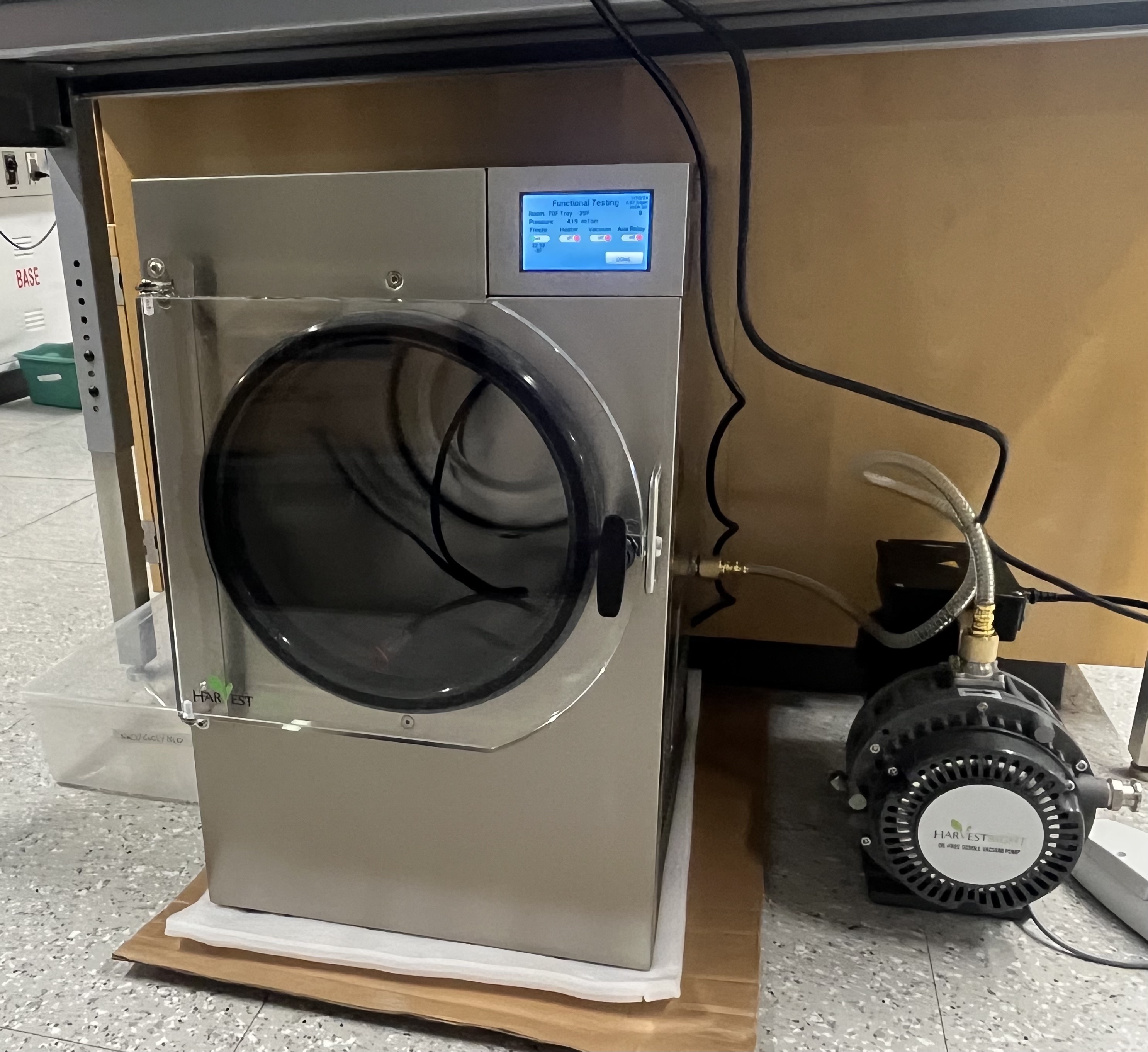
Freeze dryer
For freeze drying of aqueous solutions, a Scientific Pro Freeze Dryer from HarvestRight with an Oil-Free Pump is available. Samples are frozen to - 40 °C in a vacuum of 500 mTorr. The instrument has a capacity of ≈ 7 liters of sublimated ice. You can find more information about the instrument here.
UV lamp
An OmniCure S2000 Elite system with a High Pressure 200 Watt Mercury Vapor Short Arc lamp (irradiance up to 10W/cm2) is available on our lab. The wavelength can be set using one of the available filters, which are listed on the table below. The OmniCure R2000 radiometer can be used to monitor the UV intensity. The UV system can be connected to the MCR302e instrument to perform monitor the rheological properties of UV-curing proecesses.| Filter Type | Specification |
| S2000 Elite Filter | 400-500 nm |
| S2000 Elite Filter | 365 mm |
| S2000 Elite Filter | 320-390 mm |
| S2000 Elite Filter | 250-450 nm |
| S2000 Elite Filter | 320-500 nm |

Centrifuges
The following centrifuges available in our lab:
| Model name | Max rmp | Max g | Sample volume |
|---|---|---|---|
| Labnet Mini Centrifuge C1301 | 6000 | 2000 | 1.5/2mL vials |
| Hettich Hand centrifuge | ≈ 1000 | ≈ 3000 | 15mL tubes1 |

Phase mapping
SVM3001 Cold Properties
The SVM3001 instrument can measure the cloud point of solutions with an accuracy of 2 °C.BeNano
The 90° SLS detector on the Benano instrument can be used to measure the turbidity of samples over a temperature range of -10°C - 110°C. The temperature is set with an accuracy of ≈ 0.1 °C. Measurements can be carried out on a standard cell, whhich requires ≈ 1 mL of sample or on a micro-cuvette, requiring ≈ 50 microliters.Shaking water bath (coming soon)
Sample preparation equipment
The following equipment is available to aid with preparation of solutions:| • Roller mixer |
| • Thermoshaker |
| • Mass balance |
| • Vortexer |
Coming soon
Constant volume dialysis cells